What's Actually Inside Your Database?

Every database has to answer one question before it answers any other: when you hand it a record, where do the bytes go? The component that decides is the storage engine, and for most databases you have heard of it is built on one of two data structures. One is more than fifty years old and still the default. The other is the foundation of a growing list of newer systems.

This article covers the history that makes the two families make sense, and it deliberately stops short of explaining in detail how the second one works. That is the subject of how an LSM tree works.

Why the history matters

Storage engines look like a purely modern problem, but each design is an answer to the hardware and the workload of its time. So we start with the oldest storage format that matters here.

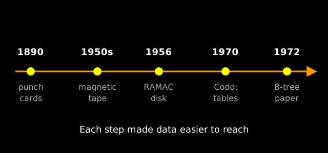
1890: holes in paper

The US Census Bureau had a problem. After the 1880 census it was collecting more data than it could tabulate, so in 1888 it ran a competition for a faster method. Herman Hollerith, a former Bureau employee, built a tabulator that worked by “reading” holes on paper punch cards. In the trial, the other two contestants needed 44.5 and 55.5 hours to prepare the data for tabulation. Hollerith needed 5.5 hours, and won the contract for the 1890 census (same Census Bureau page).

That was the state of the art in data storage: a hole is a one, no hole is a zero, and the “database” is a stack of cards.

The 1950s: magnetic tape

Computers built on vacuum tubes ran so fast that punch-card storage could not keep up. IBM’s history of magnetic tape describes how, from the early 1950s, tape greatly increased the speed of data processing and eliminated the need for massive stacks of punched cards.

Tape has one property that shapes everything that follows: it is read in order. Sequential access is the only way to get at data on a tape. If the record you want is last, you wind through everything before it. Picture a tape with a million records and the one you need is the last: you pass 999,999 others to reach it. That number is an illustration, not a measurement of any real tape drive, but the shape of the cost is real. Finding one record costs time proportional to where it sits on the tape.

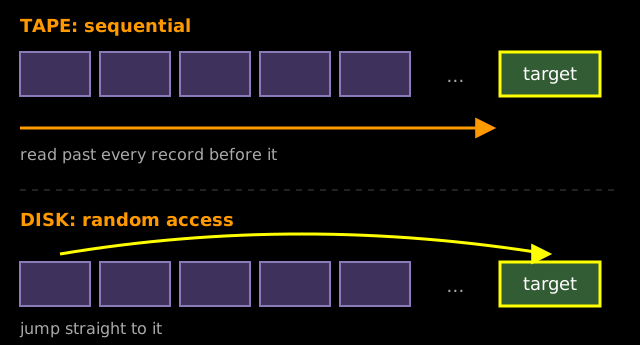
1956: the disk that can jump

IBM’s page on the 305 RAMAC calls it the first computer to use a random-access disk drive. It held 5 million binary-coded decimal characters at 7 bits per character, was the size of two kitchen refrigerators and weighed more than a ton. By today’s standards that is a few MP3 files, as IBM’s page itself notes.

The point is the access pattern. A random-access disk lets the machine go straight to a record without reading everything in front of it. No rewinding. That made it practical to keep data in an organized structure on disk and update it while the machine ran. It also set up the question the rest of this article is about: once you can jump anywhere, how should you organize what is stored so that jumping is cheap?

1970: tables

In June 1970, E. F. Codd of the IBM Research Laboratory in San Jose published A Relational Model of Data for Large Shared Data Banks in Communications of the ACM. It describes data as relations, which Codd represents as arrays where each row is one tuple and each column carries the name of its domain. Today we call them tables, rows and columns.

The idea needed something underneath it. A table is only useful if you can find one row among millions quickly, and keep finding it while new rows arrive. That takes an index structure that is fast to search and cheap to keep up to date.

The B-tree: ordered pages, shallow tree

That structure was being worked out at the same time, and not as an answer to Codd. It came from Rudolf Bayer and Edward McCreight at Boeing Scientific Research Laboratories, who were solving the general problem of indexing large files on disk. Their July 1970 report from Boeing Scientific Research Laboratories, “Organization and Maintenance of Large Ordered Indices”, describes the problem like this:

Organization and maintenance of an index for a dynamic random access file is considered.

It was later published in Acta Informatica in 1972 as Organization and Maintenance of Large Ordered Indexes, which is the citation you will usually see. 1972 is when the refereed version appeared. The report above shows the work dates to 1970, the same year as Codd’s paper.

The abstract of the report gives the key property: the scheme allows retrieval, insertion and deletion of keys in time proportional to log base k of I, where I is the size of the index and k is a device-dependent natural number. In the body of the report, k sets the page capacity: every page except the root holds between k and 2k keys. In plain terms, the index is a tree of pages, each page holds many keys in sorted order, and the number of pages you visit grows only with the logarithm of the data.

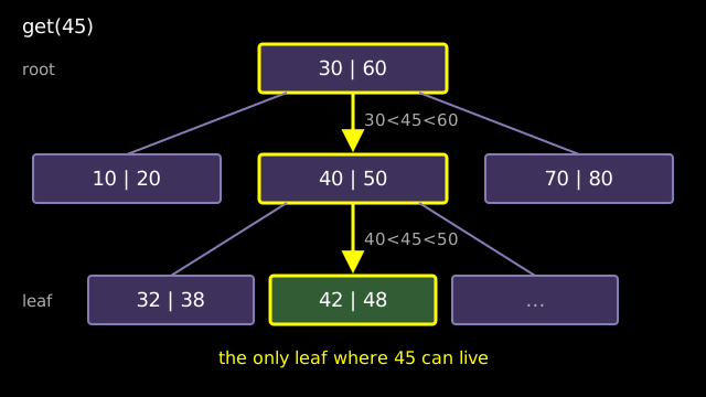
Here is the arithmetic behind “three or four hops”. If each page can hold around 100 keys, one level covers 100 keys, two levels cover about 10,000, three levels about a million and four levels about a hundred million. The 100 is an assumption for the illustration; real page capacity depends on key size and page size. The shape of the answer does not change: a lookup touches a handful of pages even in a very large table.

That is why reads are fast. Inserts keep the data sorted because each new key goes into its place in order, and page splits keep the tree balanced as it grows.

The default for fifty years

The B-tree fit the relational model so well that it became the standard answer for indexing. You can check this in the documentation of the three databases most people start with:

• PostgreSQL: CREATE INDEX creates B-tree indexes by default. The B-tree chapter says “PostgreSQL includes an implementation of the standard btree (multi-way balanced tree) index data structure.”
• MySQL: with the exception of spatial indexes, InnoDB indexes are B-tree data structures (archived copy, because the MySQL site rejects automated fetches).
• SQLite: the file format is built from b-tree pages, and its B-Tree module manages them.

One nuance: PostgreSQL keeps table rows in a heap (its docs talk about heap-only tuples) and uses B-trees for the indexes on top, while InnoDB stores the rows themselves in a B-tree, the clustered index, and SQLite stores tables as table b-trees. All three update their B-tree pages in place, which is what puts them on the same side.

The documentation supports two claims: the B-tree is the default now, and the structure is more than fifty years old.

The catch: updating in place

B-trees pay for fast reads on the write side. To insert or change a key, the engine finds the leaf page that owns it, modifies that page, and writes it back to the same place. If the page is full, it splits. The tree is updated where it lives, in place.

Then add indexes. Each index is its own structure that has to stay in sync with the table. PostgreSQL’s documentation puts it directly: after an index is created, the system has to keep it synchronized with the table, which adds overhead to data manipulation operations. With five indexes, inserting one row means storing the row and then finding, modifying and possibly splitting a leaf in each of five index trees. Not every write pays the full bill: in PostgreSQL, an update that changes no indexed column can be a heap-only tuple update that needs no new index entries. But every insert touches every index.

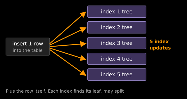
This is an acceptable price when the workload is mostly reads, or small. I am deliberately not going deeper here: why in-place updates are slow on real disks, and how much extra I/O they cause, is covered in how an LSM tree works.

The other family

So someone asked a different question. What if writes never touched the tree directly? What if you batched them and stored them separately?

That question leads to the second family of storage engines, built on the log-structured merge tree, introduced by O’Neil, Cheng, Gawlick and O’Neil in the 1996 LSM-tree paper. How it batches writes, and what it does with them afterwards, is explained step by step in how an LSM tree works.

Systems built on this idea include:

• Cassandra: its storage engine documentation says, “The architecture is based on Log Structured Merge (LSM) trees, which utilize an append-only approach instead of the traditional relational database design with B-trees” (Cassandra docs).
• RocksDB: Meta’s launch post states that data is stored in the form of a log-structured merge tree.
• LevelDB: Google’s open source key-value database library, which RocksDB builds on (repository).
• CockroachDB: through Pebble, “an LSM key-value store” (Cockroach Labs). The story of that move is in why CockroachDB replaced RocksDB with Pebble.
• ScyllaDB: uses the LSM structure to write immutable sorted string tables to disk.
• TigerBeetle: its internals documentation describes a collection of LSM trees storing objects and their indexes.

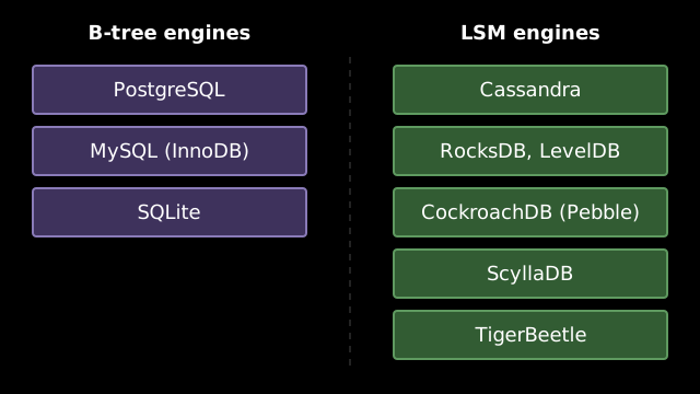
Nobody has measured how fast this side is growing, but what the list does show is that engines with very different goals, from a key-value library to a financial transactions database, chose the same family.

Why now

One reason this family is getting more attention is that cloud storage changed the economics of where data lives and what it costs to rewrite it. That claim needs numbers and a proper argument, which are in S3 and object storage for databases.

Where to go next

Two families, one question: where do the bytes go? B-trees keep the data sorted and update it in place, which makes reads cheap and writes expensive. LSM trees give up some read simplicity to make writes sequential. The next step is how an LSM tree works, followed by the RUM conjecture and why there are so many database engines.

Sources and further reading

Sources

1. B-tree storage in the default engines: PostgreSQL B-tree, MySQL/InnoDB physical structure (archived copy), SQLite B-Tree module
2. Cassandra storage engine
3. Under the hood: building and open-sourcing RocksDB and LevelDB
4. Pebble, a RocksDB-inspired key-value store (CockroachDB), ScyllaDB compaction talk, TigerBeetle docs
5. The Hollerith Machine, US Census Bureau
6. IBM 305 RAMAC
7. E. F. Codd, A Relational Model of Data for Large Shared Data Banks, CACM, 1970
8. R. Bayer and E. McCreight, Organization and Maintenance of Large Ordered Indexes, Acta Informatica, 1972

Further reading

• Bayer and McCreight, Organization and Maintenance of Large Ordered Indices, Boeing Scientific Research Laboratories report, July 1970
• IBM: magnetic tape
• PostgreSQL: index types and introduction to indexes
• SQLite database file format
• LevelDB implementation notes
• O’Neil, Cheng, Gawlick, O’Neil, The Log-Structured Merge-Tree, 1996
• Sequential access (Wikipedia)