turbopuffer: Building a Search Engine on S3
Sources (16)Watch it on YouTube ↗
Contents
In late 2022 Readwise wanted semantic search. As Simon Hørup Eskildsen, who was helping them, put it later, Readwise “was paying ~$5k/month for their relational database, but we found that vector search on the same 100m+ documents would’ve cost $20k/month+”. The feature was shelved. Vector databases of the day kept their indexes in memory, at $2 or more per gigabyte; a bucket costs about two cents.
Why not put the index in a bucket? Because a read from object storage is slow. I put an open-source graph index on a bucket and counted what one cold query did: over a thousand requests, almost all of them one after another. turbopuffer, the search engine Eskildsen went on to build, says it aims for at most three round trips on the same kind of cold query. How do you get from a thousand to three?
Who pays for idle data
Take Notion’s Q&A. A question becomes a vector, the nearest chunks are fetched from that workspace’s slice of data (a namespace), and a language model answers from them. Notion’s turbopuffer page lists 10B+ documents in 10M+ namespaces, and at any moment only some of those namespaces are being searched.
Cursor’s old setup, per the launch post, kept “every index … in memory, despite only a subset of code-bases being active at any point in time”; moving off it cut costs by 95%. Memory bills every namespace, searched or not. A bucket does not.
Three shelves, one chain
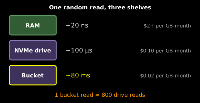
Every read lands on one of three shelves. Per Eskildsen’s napkin-math table, a read takes about 20 ns from memory, 100 µs from a local drive and 80 ms from a blob store (prices from the launch post). One bucket read costs as much time as 800 drive reads.
An embedding turns text into hundreds or thousands of numbers, and nearby points mean similar text. Checking every vector works, but takes about two seconds per million vectors even from an SSD. So search is approximate, and its quality is measured as recall: if 9 of the approximate top ten are in the exact top ten, recall@10 is 90%.
A graph you walk
The best-known approximate index is HNSW, a layered graph where each vector links to its near neighbors. A search starts at the top, hops greedily toward the query, drops a layer, and wanders the bottom layer one neighbor at a time.
Real graph indexes rarely run from a bucket. The reference library, hnswlib, allocates the whole bottom layer as one block of memory and stores each element’s neighbor list next to its vector. And the walk is a loop that cannot be read ahead: you read a candidate’s neighbor list, measure those neighbors, and only then know which list to read next. The next address is inside the read you are waiting on.
How long is the chain? On SIFT1M, a standard benchmark of a million image descriptors, I built an hnswlib index and counted. At 96% recall, one query made 76 reads in a row (about 10 in the upper layers, 66 at the bottom), and took 149 µs in memory. When a graph outgrows memory, DiskANN moves it to an SSD, with compressed vectors in memory to steer.
Now drop the same 76-read chain on each shelf, with the napkin latencies: about 8 ms on a drive, about 6 seconds on a cold bucket. Even if reading four blocks per round cut the rounds by four, the bucket would still take about a second and a half, because every round waits for the one before it. That 6 seconds is napkin math; the thousand requests I counted.
A graph on a bucket, counted
HelixDB is an open-source graph database with vector search that does put its HNSW graph on object storage. It stores everything as rows in a fork of SlateDB, a key-value store that lives in a bucket. A node’s neighbor list is one row, and its vector is another, filed in order of a SimHash fingerprint so that similar vectors share a block. The fingerprint comes from the LSM-VEC paper; the ordering is HelixDB’s layout.
I ran it on the first 100,000 SIFT vectors, on one machine with the files on local disk, and counted requests to the storage layer on a freshly started node. That is pessimistic for a cold query, since the upper layers are read through SlateDB too. A query made 367 requests on average, for 71% recall. Getting to 97% took 1,086, and never more than three were in flight at once.
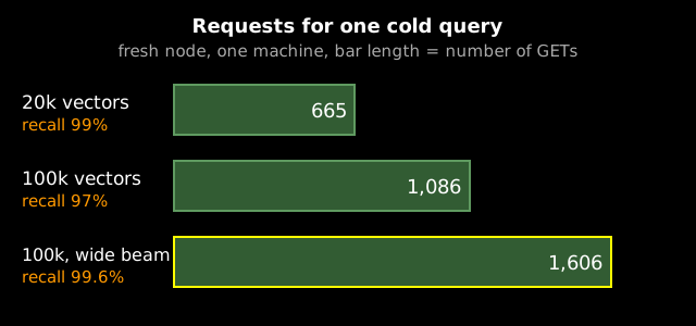
A step is not one request either: it reads a neighbor row, fingerprints and vectors from different blocks of different files, and on a fresh node each block is a request. With 20 ms injected per request, a cold query took 24 seconds (mean of 10 queries, 1,138 requests), within 6% of requests times delay: every request waited for the one before it. And the chain grows with the index: five times the vectors took 60% more requests at the same setting and lost two points of recall; holding recall at 99% took 2.4 times as many.
The graph itself is fine: with everything in an in-memory cache the same query took 29 ms and made no requests. Cold reads are what kill it. HelixDB’s own commit message says the same: with memory-only caches, a 100K-vector index on S3 thrashed the block cache and “Every HNSW hop became a serial S3 GET”. Its answer was to change the shelf: the server now always keeps a local disk cache in front of the bucket, 8 GiB by default.
These are shapes from one machine with injected latency, not real S3 and not a product benchmark.
Clusters: every address at once
Start over. Group the vectors into clusters, and give each cluster a centroid that stands in for it. A search compares the query against the centroids, picks the closest few, fetches only those clusters and checks every vector inside. This is the design of SPANN, and it changes the dependency structure: once you have read the centroids, you know the address of every cluster you need, so all those reads go out together.
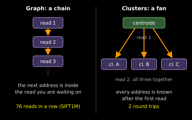
On a bucket, latency is set mostly by round trips, not bytes. turbopuffer’s post on its filtering design puts the contrast in its own words: a fully cold cluster search needs at most two round trips, unlike “graph-based ANN structures that would easily require a dozen or more roundtrips”.
The recall knob
The catch: every cluster you skip can cost right answers. I split the SIFT1M vectors into 10,000 clusters of about a hundred and measured recall against the number of clusters opened.
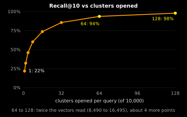
Opening one cluster finds 22% of the true top ten, 32 find 86%, 64 find 94%. Bytes read grow in a straight line, but recall flattens: from 64 to 128 clusters the vectors read double (8,490 to 16,495) for about four more points. The missing answers sit near cluster borders, so SPANN stores some border vectors in several clusters, paying space for recall.
turbopuffer’s tree in a bucket
turbopuffer is closed source, so from here on this is its own account. Its architecture docs say its vector indexes are based on SPFresh, a centroid index. Each namespace is a prefix in a bucket holding a write-ahead log and the index files: a file of centroids and big files of clusters. A query’s second index trip asks only for the byte ranges of the clusters it picked.
At a hundred billion vectors even the list of centroids is huge, so the ANN v3 post clusters the centroids too, with about 100 children per node. In its words, “the hierarchy bounds the number of round-trips to object storage to the height of the SPFresh tree”. The small upper levels stay in memory, and a one-bit copy of each vector keeps the first pass cheap, with less than 1% rechecked at full precision. At that size the post says each machine searches about 500 clusters of 100 vectors to hit its recall target, with the whole tree on local SSD.
It also checks itself: per its continuous recall post, 1% of live queries are rerun exhaustively and compared, against a 90 to 95% recall@10 target.
Keeping clusters balanced
New vectors join their nearest cluster, and data does not arrive evenly. A fat cluster slows every query that opens it, and even fresh from my build the sizes were uneven: median 93, largest 697. The usual fix is to rebuild everything. The SPFresh paper prices that for a billion-vector DiskANN graph at “a peak memory usage of 1100GB for 2 days”, and notes that Vearch rebuilds weekly.
If you know LSM trees, you have seen this choice. A global rebuild is a full compaction: rewrite everything to fix a small part. SPFresh does the small compaction, three local moves: split a cluster that passes a size limit into two, each with a new centroid; reassign vectors near the split to whichever centroid is now closest, checking only nearby clusters; merge a cluster that shrinks below a lower limit into its nearest neighbor. The paper shows a cascade of splits and reassignments always stops. In its own 100M-vector test it needed about 10 GB and 2 cores where a billion-vector rebuild needs about a thousand extra gigabytes and 32 cores, and its tail latency was 2.41 times lower than DiskANN’s.
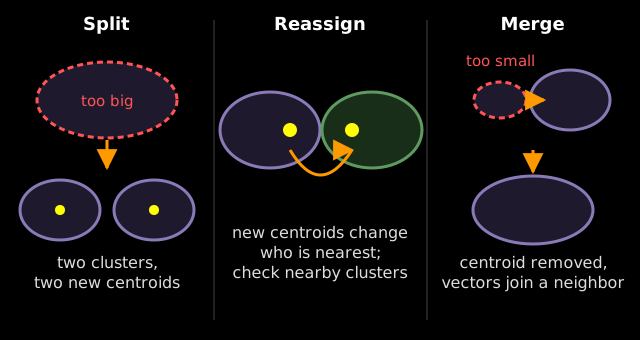
turbopuffer’s first version rebuilt the index when the log got far ahead; as Eskildsen puts it in his CMU talk, “we rebuilt the entire world”. The second runs its own, closed take on SPFresh on separate indexer nodes.
HelixDB, in the version I measured, repairs its graph inside the write: an insert starts with a search 200 candidates wide, then rewrites up to 32 neighbor lists in the same transaction. Building my 100,000 vectors took almost two hours. The first 10,000 took 39 seconds while everything fit in memory; the last 10,000 took 18.4 minutes, about 9 vectors a second. A pull request merged on October 5, 2026, after the version I measured, moves index work to a background indexer, and strongly consistent searches also check the queue.
A log in the bucket
turbopuffer’s writes skip the index entirely. Per its architecture docs, every write adds a file to a log in the namespace’s prefix, with at most one entry per second per namespace and concurrent writes batched, and the client hears OK only once the object is in the bucket (p50 of 165 ms for 500 kB). The docs mark a compare-and-swap commit point and an index cursor showing how far the index has caught up; in the same talk, Eskildsen says log files are committed into a manifest with that compare-and-swap.
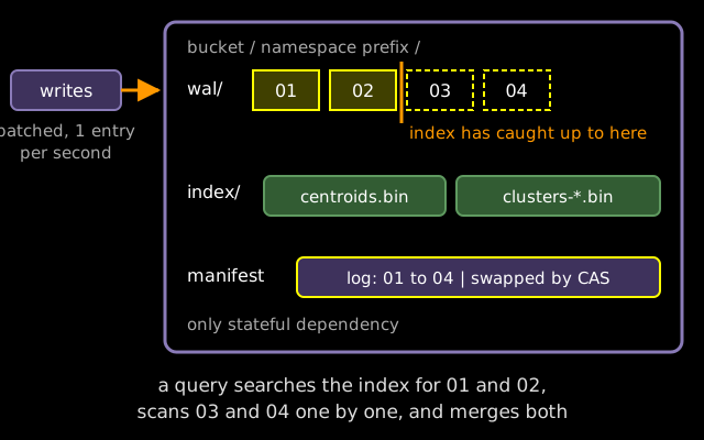
Before answering, a query asks the bucket whether the manifest changed: a conditional read of about 10 ms that sets a latency floor for consistent reads. Eventual consistency skips it. Data not yet indexed is searched exhaustively from the log and merged with what the index found. That is a memtable plus sorted runs read path with the recent part stored in the bucket. When more than 128 MiB is waiting to be indexed, new writes wait before they show up.
Underneath, Eskildsen says in the talk, the indexes are key-value pairs in an LSM with about the simplest tiered compaction you can imagine, run by the indexer nodes.
In September 2026 turbopuffer announced a v3 that stops keying everything by the vector’s cluster address, because splitting a cluster then moves the document and every index entry pointing at it: “Updating just one vector can move hundreds of attributes and their indexes.” The vector index becomes one secondary index among others. As of November 2026 its nightly benchmark shows v3 faster than production on most queries (p90 hot full-text 20 ms against 38, hot vector 21 against 41), with only some hot count queries slightly slower. It is not in production yet, and the page’s footnote says “we do not expect v3 to significantly reduce latency for cold vector queries”.
Counting a cold query
A cold query, as the docs describe it: one trip for the namespace’s metadata, one for the filter index, the centroids and the not-yet-indexed log in parallel, and one for the clusters. Large indexes can need a fourth.
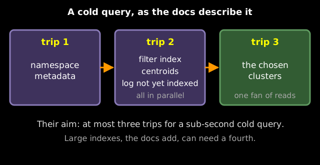
Three is a design rule rather than a result: the launch post says “we aim to limit it to a maximum of three roundtrips for sub-second cold latency”, and the planner trades an extra trip against fetching more bytes in a trip it is already making. The docs call the 3 to 4 trips “as little as ~400ms” and give medians for 1M documents: 874 ms cold and 14 ms warm.
Next to my count of 1,086 dependent requests on a fresh HelixDB node, this is not a ranking: one is my measurement, the others are turbopuffer’s target and median. What they share is a shape: a graph pays for a chain of dependent reads, a tree of clusters for its height.
Who keeps what warm
What remains is how much to keep warm. In turbopuffer, query nodes are caches in memory and on NVMe, and only the bucket holds state, so any node can serve any namespace and a dead node costs only its cache. Cold queries happen when a namespace sat idle for hours or its node died.
Amazon S3 Vectors quotes under a second for infrequent queries and about 100 ms or less for frequent ones. Notion hides the cold query: opening a dialog that may search fires a prewarm query for that namespace, which is free if it is already warm. You can also pay to pin a namespace on reserved drives, billed by the hour, with a break-even around 10 queries per second. At the far end, Perplexity’s CobbleDB never goes cold: for the pages Perplexity chooses to serve, its hot store keeps the passages and their embeddings on NVMe, in three replicas.
When to pick it
By its own account, turbopuffer fits first-stage retrieval, where you cut millions of documents to a few candidates for your own code to rerank, over many namespaces that sit mostly idle, with writes that can wait. Skip it if every read must be consistent in under 10 ms (eventual consistency is the escape hatch), if you need transactions, or if it must be open source you run yourself.
Sources and further reading
Sources
- turbopuffer: fast search on object storage, Simon Hørup Eskildsen, updated March 5, 2026: Readwise, Cursor, the three-round-trip aim.
- turbopuffer architecture: WAL, manifest, SPFresh-based index, cold and warm medians.
- turbopuffer guarantees, tradeoffs and limits: bucket as only state, no general transactions, 128 MiB limit, 10 ms floor, hours in cache, when to pick.
- Notion on turbopuffer: 10B+ documents, 10M+ namespaces, prewarm.
- ANN v3: 100 billion vectors: tree of centroids, round trips bounded by height.
- Native filtering: at most two round trips against a dozen for graphs.
- Continuous recall: exhaustive timing, recall@k, 1% sampling.
- RIP, vector database and the v3 page: v3 and its nightly benchmark, as of November 2026.
- Warm cache and pinning docs.
- napkin-math: the latency table.
- hnswlib and the HNSW paper.
- DiskANN, NeurIPS 2019.
- SPANN, NeurIPS 2021 and SPFresh, SOSP 2023.
- LSM-VEC and HelixDB, the disk-cache commit and PR #1156.
- CMU Database Group talk by Simon Hørup Eskildsen: the first version’s rebuilds, the LSM underneath.
- Amazon S3 Vectors GA and Perplexity CobbleDB.
My own measurements (hnswlib on SIFT1M, flat clusters on SIFT1M, HelixDB on the first 100,000 SIFT vectors) were run on one machine, and the HelixDB numbers use a local filesystem with 20 ms injected per request.
Further reading
- SlateDB: what if S3 were your only disk for the bucket-native key-value store HelixDB sits on.
- S3 and object storage for databases for the price and request model behind the shelves.